Muon decay measurement with Red Pitaya

Abstract: In this article, we present the design of a cosmic ray detector built around a plastic scintillator coupled with a photomultiplier. The pulses generated by cosmic ray interactions are captured using the Red Pitaya microcomputer. Thanks to its high sampling rate and the capability for software-based pulse processing, the Red Pitaya enables precise measurement of the decay time of muons that come to rest within the scintillator.

Introduction

The project we propose in this work, partially described in previous posts on this site, consists of a cosmic ray detector based on a plastic scintillator coupled with a photomultiplier. Numerous cosmic ray detection projects have appeared in the scientific literature, particularly in the context of educational activities. Notably, we were inspired by the commercial product developed by TeachSpin. However, our project adopts a predominantly DIY approach, leveraging open, widely available, and low-cost technologies.

The readout electronics are kept minimal, consisting of a trans-impedance amplifier optionally followed by a fast comparator. The key innovation lies in the data acquisition system, which uses the Red Pitaya microcomputer. The Red Pitaya, with its 125 Ms/s sampling rate and 14-bit ADC, ensures precise pulse timing and enables measurement of the decay time of muons that stop and decay within the scintillator.

Whenever possible, components are low-cost, open-source, and home-built. The only exception is the detector probe, which consists of a plastic scintillator coupled with a photomultiplier. However, both the scintillator and photomultiplier can be sourced easily and affordably from the online surplus market.

This project aims to make cosmic ray detection accessible to a wider audience, combining educational value with cutting-edge yet affordable technology.

Theoretical and Historical Notes

The μ lepton (muon), the primary component of secondary cosmic rays, is an elementary particle with a spin of 1/2, a mass of 105.65 MeV, and a half-life of approximately 2.2 μs. Muons are produced in the upper atmosphere, predominantly through the decay of π particles, which are themselves created during collisions between primary cosmic rays and atmospheric gas nuclei. Upon production, muons exhibit relativistic speeds, and due to time dilation, they can reach sea level despite their short half-life.

The muon was the first unstable elementary particle to be discovered. At the time of the pioneering experiments conducted by Bruno Rossi, Franco Rasetti, and others, the only fundamental particles known were the photon, electron, positron, proton, neutron, and neutrino. Since then, dozens of particles and antiparticles have been identified, most of which are unstable. In fact, among all particles observed as isolated entities, only photons, electrons, protons, neutrons, neutrinos, and their antiparticles have longer lifetimes than muons. Even the neutron, when free, undergoes beta decay with an average lifetime of approximately 15 minutes.
It is known that the muon decays into an electron, a muon neutrino and an electron antineutrino, as shown in Fig.1.

Figure 1 – Decay scheme of the Muon into an Electron and two Neutrinos

The times of muon decay are described mathematically in a simple way. Suppose we have a number N(t) of muons at time t. If the probability that a muon decays in a short time interval dt is λdt, where λ is the constant that characterizes the decay rate of the muon, then τ = 1/λ is the time constant of the decay and the number of muons decreases with the exponential law:

N(t) = N₀e^(-λt)

N(t) is the number of muons still existing at time t
N₀ is the number of muons at time t = 0
The muon mean life τ = 1/ λ

However, we do not have a group of muons which are decaying. Instead, we detect decays following muons that enter the detector randomly, typically one at a time. Even in this case, however, the decay time distribution follows a simple exponential law. Since the decay time is distributed with an exponential law, it is not important that the muon whose decay we record was produced in the detector rather than in the upper atmosphere: an exponential function always appears the same no matter when it is examined, its “exponential shape” does not change over time.

Method of Measurement of Decay Time

The detector, composed of a plastic scintillator coupled with a photomultiplier tube (PMT), is schematized in Fig.2. The detector generates numerous pulse signals every second. Many of these signals originate from electronic noise within the device itself or from environmental radioactivity. These unwanted signals are filtered out by the readout electronics, as described in the section detailing the experimental apparatus.

The remaining signals primarily correspond to muons passing through the scintillator crystal, which are detected and counted by the apparatus. Among these events, the most interesting are those caused by muons entering the scintillator with kinetic energy significantly lower than the average value. These muons lose their energy by transferring it to the scintillator, eventually coming to a complete stop within the crystal. Upon stopping, they deposit the final portion of their kinetic energy —typically around 40 MeV, depending on the scintillator material— into the scintillator. This deceleration produces an initial light pulse, which is detected by the PMT.

Figure 2 – Schematic showing the generation of two light pulses (blue arrows and green arrows) used in the determination of the muon lifetime. The first pulse of light comes from the slowed-down muon (dotted line) while the second comes from the electron produced by the decay (wavy line)

The muons that stop within the scintillator remain there for a relatively long time, on the order of microseconds. Each muon decays into an electron (or a positron, in the case of an antimuon) along with a neutrino and an antineutrino. The entire rest energy of the muon (106 MeV) is converted into the kinetic energy of these three particles. On average, the electron (or positron) receives about one-third of this energy, approximately 35 MeV, while the remaining energy is carried away by the two neutrinos. However, since neutrinos are not detectable by our instrument, only the electron contributes to the observable signal.

As a charged particle, the electron causes ionization as it travels through the scintillator, generating a second light pulse. This second pulse is detected by the PMT and is crucial for measuring the time interval between the initial and secondary pulses. The distribution of these time intervals for a set of muon decays represents the physical quantity of interest, allowing us to determine the muon’s decay time.

Experimental Apparatus

The experimental apparatus consists primarily of a scintillation detector, electronics for amplifying the pulses produced by the PMT, and a Red Pitaya microcomputer. The Red Pitaya records the pulses, counts them, and measures the time intervals between successive pulses. The collected data is subsequently processed using the ROOT software, which is utilized for data fitting and visualization.

Photomultiplier and Plastic Scintillator

To optimize the efficiency of muon detection, the BC412 plastic scintillator was selected due to its affordability and widespread availability. This scintillator is particularly well-suited for detecting charged particles, such as muons and electrons. The dimensions of the crystal, shown in Fig. 3, are 114 mm in thickness with a surface area of 119 mm². The primary material of the scintillator is polyvinyl toluene, which has a density of 1.023 g/cm³ and emits light in the range of 400–520 nm, with a peak emission at 434 nm. The light pulse generated by the BC412 has a full width at half maximum (FWHM) of 4.2 ns, which is short enough to avoid interference with subsequent readings by the PMT. The detailed properties of the scintillator are summarized in Table I.

According to literature data, for muons with energies of approximately 100 MeV, the material’s stopping power is estimated to be around 3 MeV/cm. Given the crystal’s thickness and the muon’s trajectory — either vertical or slightly inclined — the total energy loss is approximately 35–40 MeV. The BC412 plastic scintillator has a quantum yield of 11,400 photons/MeV, implying that a light pulse produced by a muon consists of approximately 300,000–400,000 photons. Similarly, the light pulses generated by the electrons from muon decay are of the same order of magnitude. These high photon yields result in pulses of significant amplitude when recorded by the PMT.

Bicron BC412 plastic scintillator – www.ebay.it/itm/Bicron-BC412-Round-Scintillator-Plastic-for-1-1-2-inch-PMT-detectors-1-6-X2-25-/253211792569 – eBay cost 40 €

Scintillator data
Type	BC412
Material	polyvinyl toluene
Dimensions	114 mm x 119 mm2
Density r	1,023 g/cm3
Emission spectrum	400 nm – 520 nm
Emission maximum wavelength	434 nm
Pulse duration (FWHM)	4,2 ns
Quantum yield	11400 photons/MeV
Stopping power at 100 MeV	~3 MeV/cm

Table I – Scintillator data

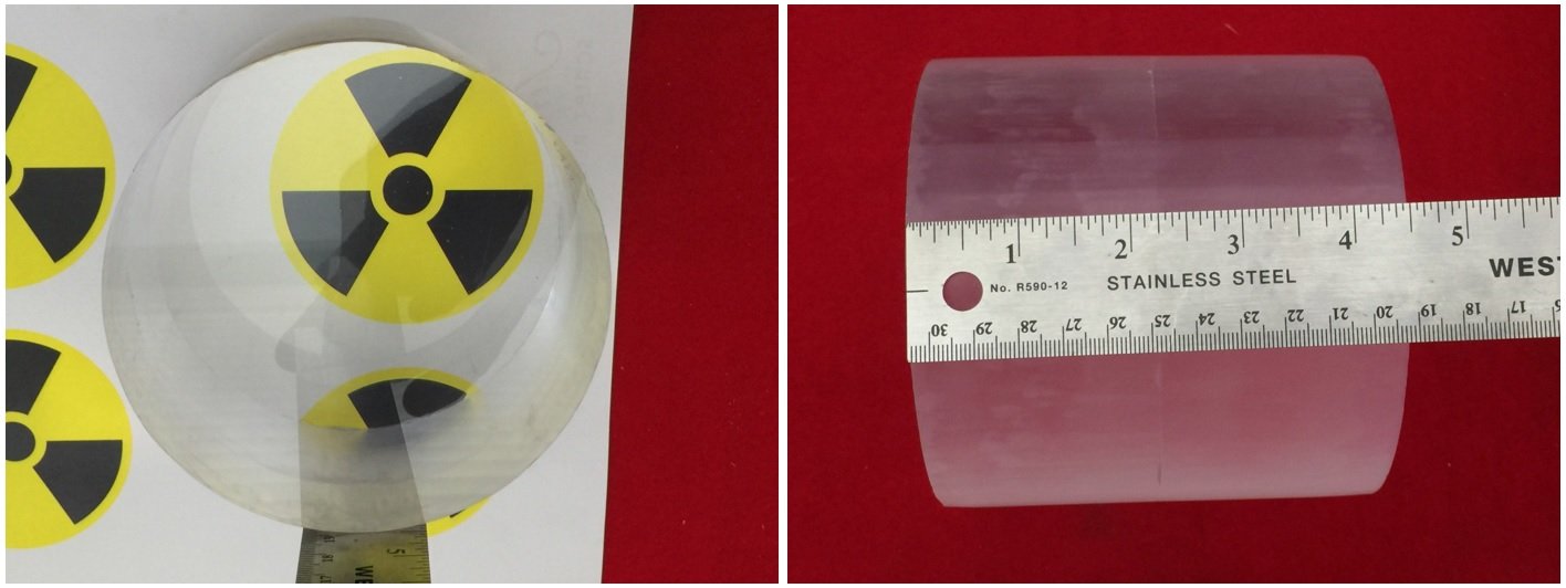Figure 3 – Plastic scintillator

The photomultiplier tube (PMT) used in this setup is the Hamamatsu R6233 model, a general-purpose device featuring a 76 mm diameter Bialkali-type photocathode. It is sensitive to light within the 300–650 nm range, with peak sensitivity at 420 nm. Although this PMT is not particularly fast, it has a response time of 9.5 ns and a transit time of 52 ns. Consequently, the pulses produced by the PMT are expected to have a duration of approximately 50 ns. This duration, however, is sufficiently short to ensure that the temporal precision of pulse acquisition is not compromised. The detailed specifications of the photomultiplier tube are listed in Table II.

Hamamatsu photomultiplier R6233 – www.ebay.it/itm/261922622140 – eBay cost 200 €

Photomultiplier data
Model	R6233 Hamamatsu
Photocathode	Bialkali
Photocathode diameter	76 mm
Sensitivity spectrum	300 nm – 650 nm
Wavelength maximum sensitivity	420 nm
Response time	9,5 ns
Transit time	50 ns

Table II – Photomultiplier data

The photomultiplier tube (PMT) is completed with a resistive divider on the dynodes. To ensure optimal optical coupling between the refractive indices of the scintillator and the borosilicate glass of the PMT, the two components are joined using silicone grease, effectively minimizing reflections at the contact surfaces.

The scintillator is then wrapped in white Teflon tape, which reflects inward any light that would otherwise escape the crystal without reaching the PMT. This increases the overall detection efficiency. Finally, the entire assembly is enclosed in a dark, opaque sheath—such as a heat-shrink sleeve—to prevent ambient light from reaching the PMT, as illustrated in Fig. 4.

Figure 4 – PMT coupled to scintillator

The photomultiplier tube is powered by a high-voltage HV circuit based on the PMT adapter Theremino. Everything is placed inside a metal container, protected from ambient light, as shown in Fig.5. The pulse signal is read through a coupling capacitor to isolate the high-voltage line from the signal line. The HV circuit is powered via a normal 5 V voltage.

Figure 5 –  Detector

Readout Electronics

The pulses produced by the PMT are sent to a signal processing chain consisting of:

• Transimpedance amplifier;
• Fast comparator;

The current pulse (of negative polarity) generated by the PMT is fed into a transimpedance amplifier (TIA) circuit (Fig. 6), which converts the current pulse into a voltage pulse. To preserve the shape of the original signal produced by the PMT, a very fast operational amplifier is required. For this reason, the TI OPA354 operational amplifier was selected, as it ensures a rise time of only 2 ns. The signal produced at the output of the amplifier is inverted relative to the input, resulting in a signal that swings positively from the ground (GND) level to a maximum of approximately 2 V.

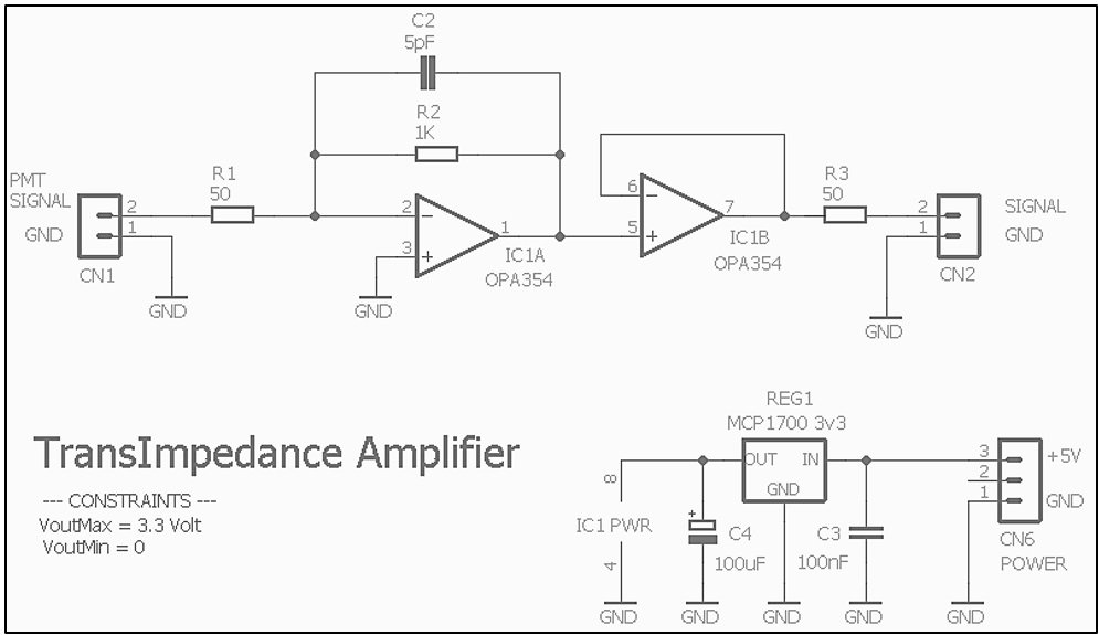
Figure 6 – TIA amplifier scheme

The amplified signal is fed into a fast comparator with hysteresis (Fig. 7), implemented using the LT1016 chip from Analog Devices, which ensures switching times of only 10 ns. The comparator, which features an adjustable threshold, is designed to produce a square pulse signal corresponding to the pulses generated by the PMT. By adjusting the threshold, it is, therefore, possible to selectively detect the pulses produced by muons and exclude the “noise” from environmental radioactivity. This is because muons typically generate pulses of higher amplitude, while pulses from background radioactivity remain below 100–200 mV. The threshold was set to 200 mV. With this threshold, the counting rate from muon detection is approximately 5–7 pulses per second, equivalent to 250–300 counts per minute (CPM).

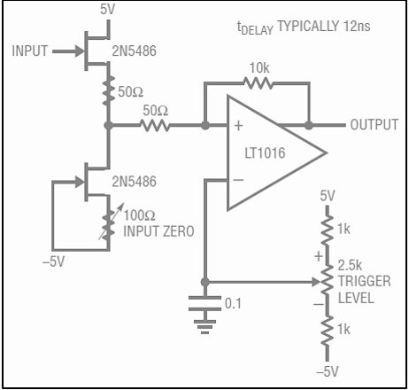Figure 7 – Fast comparator scheme

The readout electronics, constructed on prototype bases, are housed in an aluminium enclosure, as shown in Fig. 8 and Fig. 9. Two external outputs are provided via BNC connectors: one for the amplified signal and one for the signal generated by the fast comparator. Additionally, the enclosure features a potentiometer for adjusting the comparator threshold, as well as another BNC connector for measuring the set threshold value.

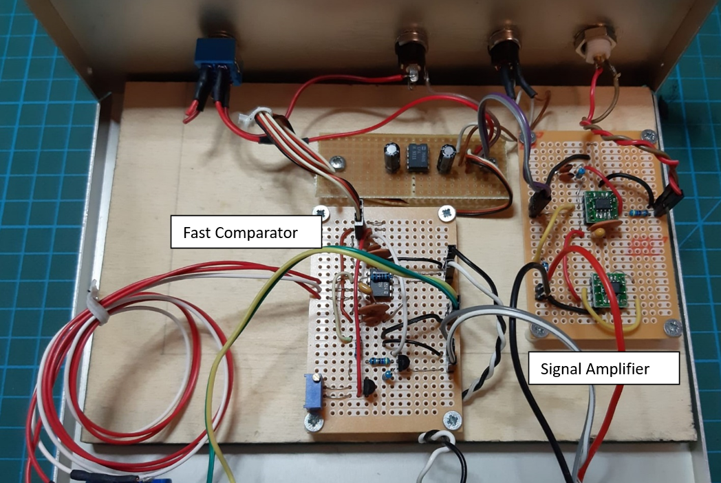Figure 8 – Internal view of the electronics

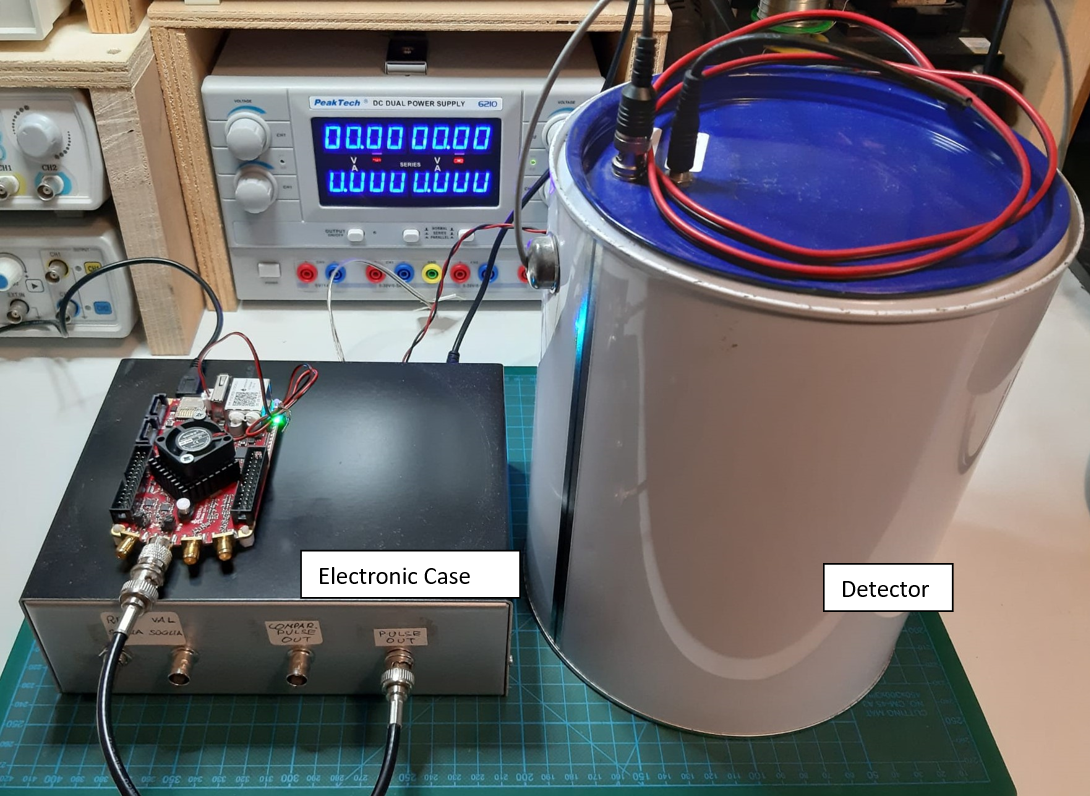Figure 9 – Complete apparatus with the detector and Red Pitaya card

Red Pitaya Data Acquisition Tool

For impulse acquisition and processing, we chose to use the Red Pitaya board. This circuit board is a Linux-based microcomputer equipped with two 125 MS/s RF analog inputs and two 125 MS/s RF analog outputs, each with a 50 MHz bandwidth. The analog I/Os are connected to analog-to-digital converters (ADC) and digital-to-analog converters (DAC), both with 14-bit resolution. The preloaded software includes several applications, such as an oscilloscope, spectrum analyzer, and signal generator. One of the main advantages of this board is its reprogrammability, allowing users to customize its functionality, as all I/O ports are connected to a shared FPGA. Fig. 10 shows the board and its interfaces, while Fig. 11 illustrates how one of the board’s analog inputs is connected to the amplifier output to acquire the impulsive signal generated by the muon detection in the scintillator.

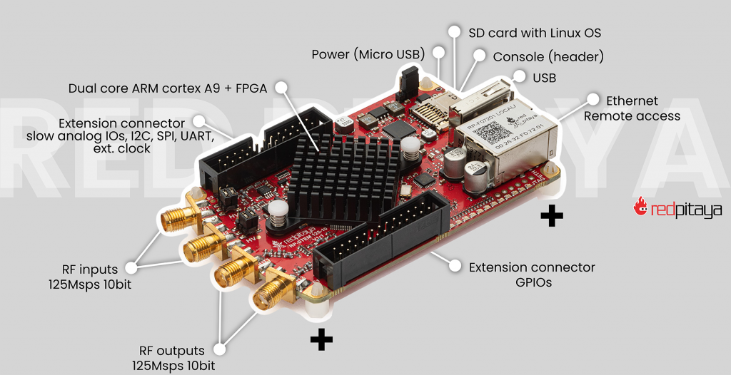
Figure 10 – Red Pitaya board with connectors and other details

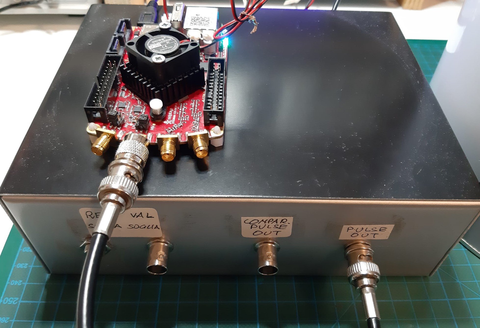
Figure 11 – Red Pitaya acquisition board connected to the signal amplifier

Impulse Analysis

Fig. 12 shows the typical pulses produced by the PMT and after the readout electronics. The pulses generated by the PMT have an amplitude greater than 200 mV and a duration (FWHM) of 40 ns. After passing through the transimpedance amplifier, the pulse amplitude increases to 1–2 V, while the duration remains the same. Fig. 13 illustrates a typical pulse acquired by the Red Pitaya board. The trigger level must be set high enough to exclude spurious pulses with smaller amplitudes, such as those caused by environmental radioactivity or device noise. This ensures that only pulses produced by the actual interaction of muons with the scintillator are acquired.

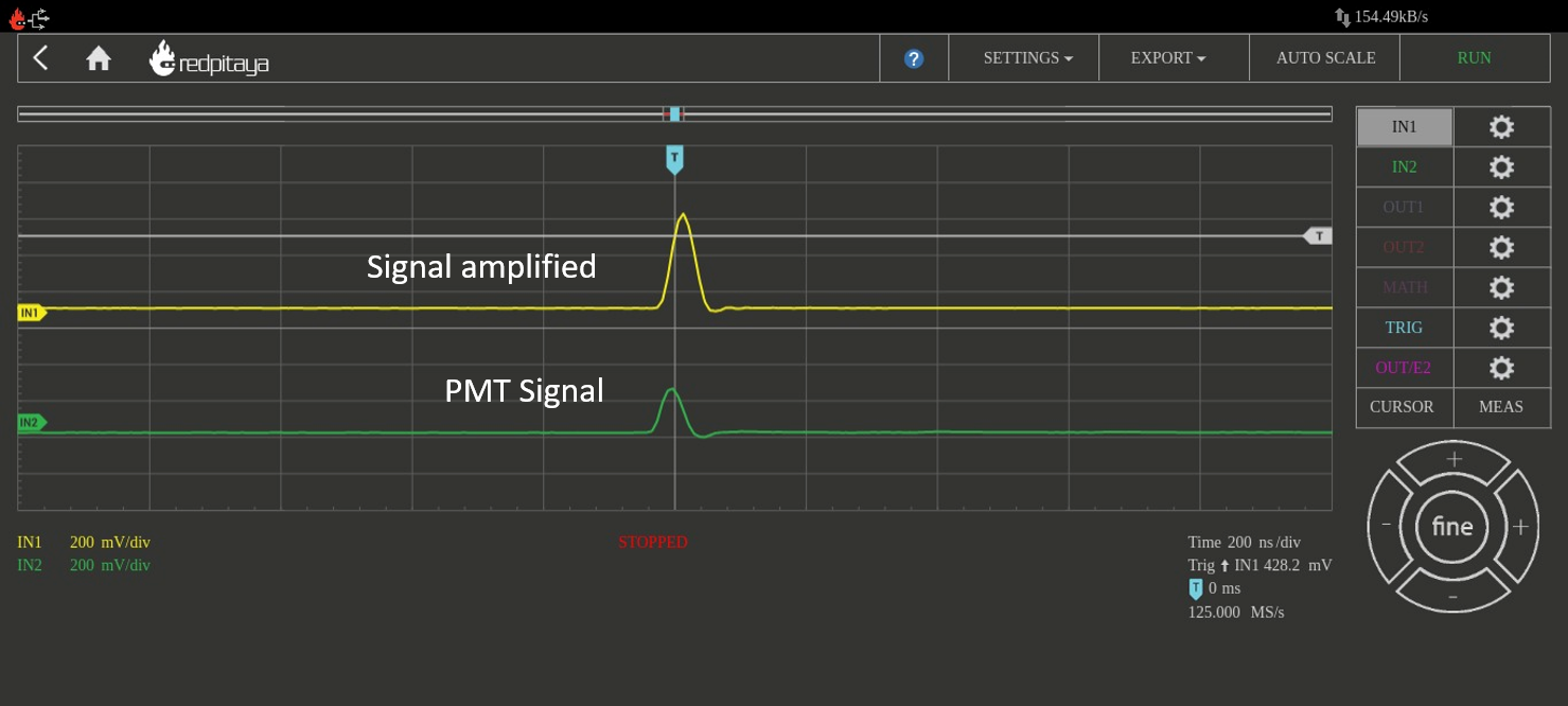Figure 12 – PMT pulse (in green) and pulse after amplification (in yellow)

The pulses of interest have a relatively high amplitude (>100 mV), making them easily distinguishable from others with lower amplitudes. As explained in previous sections, the pulses we are focused on are those produced by the decay of a muon inside the scintillator. These events can be identified because they consist of two pulses separated by a short time interval (on the order of microseconds), as shown in Fig. 14. The first pulse corresponds to the muon’s interaction with the scintillator, while the second pulse is produced by the electron/positron generated in the muon’s decay. Although the amplitude of the second pulse is slightly smaller, it remains on the same order of magnitude as the first.

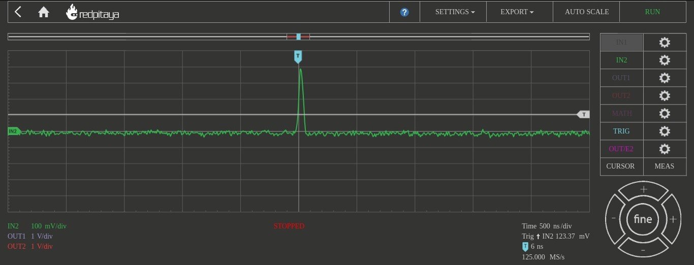Figure 13 – Pulse acquired with Red Pitaya board

Figure 14 – Examples of pulses caused by the passage of a muon and its subsequent decay into an electron. The electron has high kinetic energy and therefore leaves a trace of similar width to that of the muon. In the first case, the time interval is approximately 1600ns, and in the second case, it is approximately 5600ns.

Data Acquisition and Processing

To acquire the events of interest and extract the time interval between the two pulses, we developed a C software that utilizes the Red Pitaya APIs. The process begins by acquiring the digitized sample from the analog input. This sample consists of a 16K vector of values, which represent the signal sampled by the ADC. The vector is then scanned for pulses, and if a pair of pulses with amplitudes within the expected range is detected, the time interval between the two pulses is measured and recorded. The device has been running continuously for several days to accumulate a large number of events.

The data were then processed using ROOT, which was used to construct histograms of the time interval distribution and to determine the fitting parameters with an exponential function. The graphs, presented in both linear and semi-logarithmic scales, are shown in Fig. 15 and Fig. 16. The maximum time acquired is 20 μs. The time interval from 0 to 20 μs was divided into 200 bins, each 0.1 μs wide. The first two bins (0.2 μs) were excluded due to higher uncertainty in such short time intervals. The total number of recorded events was 10,024. Based on these data, the exponential function that best fits the collected data was determined. An offset was also included in the fitting function to account for events that were temporally close but not correlated.

f(x) = off + amp x e^-t/τ

From the fitting of the data we obtain the lifetime of the muon which is :

τ = 2.100 ± 0.027 μsec

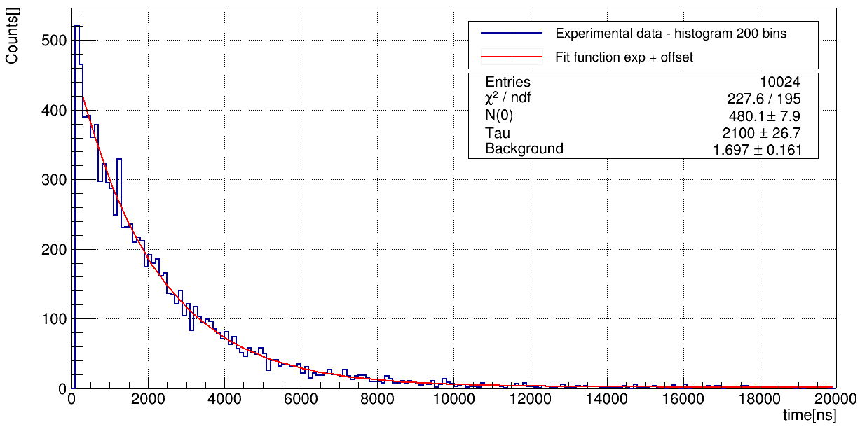Figure 15 – Linear scale histogram of time intervals and exponential fitting

Figure 16 – Logarithmic scale histogram of time intervals and exponential fitting

Muons or Antimuons?

The muons we detect and whose lifetimes we measure can be either muons (negatively charged) or antimuons (positively charged). The muons that slow down and stop in the scintillator can bind to nuclei in much the same way as electrons do. Since the muon is not an electron, the Pauli exclusion principle does not prevent it from occupying an atomic orbital already occupied by an electron. These bound muons can then interact with the protons in the nuclei, producing a neutron and a neutrino: μ^– + p -> n + ν_μ
This interaction can occur before spontaneous decay. There are therefore two different ways for a muon to “disappear”: spontaneous decay and interaction with a proton, which means that the effective lifetime of muons inside matter is slightly less than their lifetime in a vacuum. For antimuons, which are positively charged, this does not occur because they do not form bound states with nuclei, this second interaction mechanism is therefore not available, so their lifetime is not disturbed by interactions with matter.
The lifetime we measure with our apparatus, being an average over both particles, will therefore necessarily be a little less than the lifetime of the muon in a vacuum, equal to τ_μ =2.19703 ± 0.00004 μsec. As regards the interaction of the muon with matter, we can consider the plastic scintillator as consisting mainly of carbon, for which the lifetime has been carefully measured and is τ_c = 2.043 ± 0.003 μsec. We therefore have the following data:
For antimuons – without interaction: τ⁺ =2.19703 ± 0.00004 μsec
For muons – with interaction: τ^– =2.043 ± 0.003 μsec

The value we observe should be between these two values. Assuming that at ground level the number of muons is equal to the number of antimuons (from the scientific literature it is clear that there is a small prevalence of positive muons, but for our level of analysis we can assume they are equal) the average decay time can be calculated in the following way:

1/τ = 1/2(1/τ⁺ )+ 1/2(1/τ^–) ->  τ = 2.117 μsec

The value obtained in our measurement is τ = 2.100 ± 0.027 μsec, which is therefore in good agreement with the expected value.

Conclusions

The apparatus described in this article has proven to be a highly efficient muon detector. The electronic components are straightforward, and the use of the Red Pitaya acquisition card enables easy observation of the pulses generated by muons passing through the plastic scintillator. With “ad hoc” software based on the Red Pitaya APIs, the pulses can be easily recorded for subsequent analysis. In this project, we focused on analyzing the pulses to identify those corresponding to the muon’s decay. Using this approach, we successfully acquired over 10,000 decay events, allowing us to obtain an excellent estimate of the particle’s lifetime.

If you liked this post you can share it on the “social” Facebook, Twitter or LinkedIn with the buttons below. This way you can help us! Thank you!

Donation

If you like this site and if you want to contribute to the development of the activities you can make a donation, thank you!